The Research: Seasonality Revisited
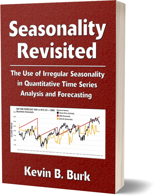
Seasonality Revisited: The Use of Irregular Seasonality in Quantitative Time Series Analysis and Forecasting

Abstract
This monograph revisits the theory of seasonality by asserting that seasonality is a quality of time, and that the calendar and clock are not the only ways to measure time.
If seasonality is a quality of time, then the seasons of a time series are defined by the divisions of time within the seasonal model and not by patterns of peaks and troughs in the data itself. Every season has an effect that can be quantified. Cohen’s d provides an objective metric to quantify the magnitude of the effect of any season in relation to the mean value of the calendar year. This allows for comparison of seasonal effects within a seasonal model, between different seasonal models, and even between seasonal models applied to different data sets.
The historic variance of the effect sizes can be quantified and used to anticipate the predictive value of a season. The more consistent the historic effect size is, the lower the variance, and the greater the expectation that the seasonal pattern will continue in the future.
Each historic season has a mean value, and seasonal forecasts that predict the mean value for future seasons can be generated using a moving average of non-contiguous historical data, considering historical values of the season itself. These seasonal forecast signals can be combined with traditional forecasts to create a hybrid forecast that includes the seasonal influences.
Because the seasonal forecast is separate from the traditional forecast, it is also possible to incorporate only the seasonal data of seasons with the lowest variance and the greatest expectation that they will improve the accuracy of the final forecast. This is called Targeted Seasonality.
The seasonal models of the calendar and the clock are based on the cycles of the Sun as observed from the Earth. These are examples of regular seasonality. This study introduces seasonal models based on the observed speed and direction of the planet Mercury. These are examples of irregular seasonality.
The quantified significance of Calendar Month seasonality is used as the baseline of comparison to evaluate the potential significance of the irregular Mercury-based seasonal models. The seasonal models are compared across three extensive and unrelated data sets: Transportation On-Time Performance, Car Crash, and Financial Market data. The Mercury-based irregular seasonal models showed a far greater percentage of significant seasons than the Calendar Month model. The ability to compare and contrast seasonal effects in this way demonstrates the practical value of the effect- and variance-based approach to quantifying seasonal influences. It also confirms that irregular seasonal models can reveal patterns in time series data that are otherwise undetectable.
To test the value of incorporating irregular seasonal influences in time series forecasting, 76 quarterly forecasts covering a 19-year period from 2000–2018 were generated for each of 430 individual financial data sets (10 stock market indexes, 379 individual stocks, 21 commodities, 10 interest rates and bonds, and 10 currency exchange rates). The aggregate accuracy of twelve different forecast models was then ranked and compared with both mean absolute percentage error (MAPE) and root mean square error (RMSE) The forecast models include five non-seasonal traditional forecast models (ARIMA, ESM, Holt, Mean, and Naïve), the seasonal forecast generated using the M15 Sign + Speed seasons, and six hybrid seasonal forecasts that combine the seasonal forecast data with the forecast data of each of the traditional forecast models.
If the forecasts that include the irregular seasonal data are more accurate than the non-seasonal forecasts by a significant percentage (60% or greater), then these irregular seasonal models have clear value in quantitative time series forecasting.
Two different methods, designated, E3 and M3, were used to generate the seasonal forecasts for the entire data set. For the forecasts that used the E3 model, the hybrid seasonal forecasts were more accurate than their non-seasonal counterparts 71.30% of the time (MAPE) and 66.93% of the time (RMSE). For the forecasts that used the M3 model, the hybrid seasonal forecasts were more accurate than their non-seasonal counterparts 74.37% of the time (MAPE) and 72.33% of the time (RMSE). This clearly demonstrates that including the irregular seasonal influences has a significant chance of improving the accuracy of the forecast.
Finally, to test the hypothesis that the lower the historical variance of the effects of a season, the greater its value in improving the accuracy of forecasts, the forecast accuracy for both forecast methods were evaluated considering only the seasons in each data set that met the threshold of significance for variance. In every instance, the targeted results were more accurate than their non-targeted counterparts. This strongly suggests that the historical variance of the effects of a season correlates to the value of using that season in time series forecasting.
The conclusions of this study are that there is clear and consistent value in this new approach to seasonality, both with quantitative time series analysis and with quantitative time series forecasting. These discoveries are worth further serious consideration and exploration.
Purchase Seasonality Revisited on Amazon.com
Resources: Tableau Workbooks
Packaged Tableau Workbooks

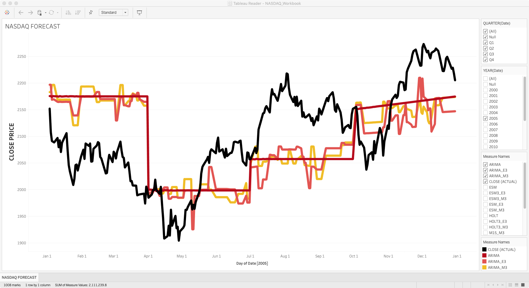
This ZIP file contains packaged Tableau workbooks to explore the M30 and M15 Mercury seasonal models and the various forecast graphs for 13 data sets from the Financial Forecast study.
To view and interact with these files, you will need at least Tableau Reader 2021 (download here for free).

